This post is an adaptation from Using databases with Shiny.
Shiny apps are R’s answer to building interface-driven applications that help expose important data, metrics, algorithms, and more with end-users. However, the more interesting work that your Shiny app allows users to do, the more likely users are to want to save, return to, and alter some of the ways that they interacted with your work.
This creates a need for persistent storage in your Shiny application, as opposed to the ephemeral in-memory of basic Shiny applications that “forget” the data that they generated as soon as the application is stopped.
S3 buckets are a form of persistent storage for web applications. Managing S3 buckets (with write access) for use with a web application is easier than managing a databases, as you won’t find yourself needing to define tables, secure data, and manage connections. In particular, working with Apache Arrow noticeably simplifies reading from and writing to S3 buckets from different providers such as AWS, DigitalOcean, and others.
This post provides some tips, call-outs, and solutions for using S3 for persistent storage with Shiny. In my case, I rely on an elemental Shiny app and served on the DigitalOcean App platform.
Databases & Options for Storage
Dean Attali’s blog post on persistent storage compares a range of options for persistent storage including databases, S3 buckets, Google Drive, and more.
For my application, I anticipated the need to store and retrieve sizable amounts of structured data, so using a S3 and the RStudio image that I created to read the data from a server in the same network as the S3 bucket (i.e. improved reading/writing speed) seemed like a good option.
Since I was hosting my application on the DigitalOcean App Platform, I could create an S3 bucket with just a few button clicks and I have the advantage that the aforementioned image already included Shiny and Shiny Server. This solution offers some significant benefits in terms of security, including the option of serving/editing my app over HTTPS and using an image that already restricts root’s SSH access and bans repeated failed login attempt.
For more information on different options for hosting Shiny apps and some insight into why I chose Digital Ocean, check out Peter Solymos’ excellent blog on Hosting Data Apps.
Creating an S3 bucket
To create an S3 bucket (i.e. a Space in DigitalOcean terminology) for my application, I simply went to:
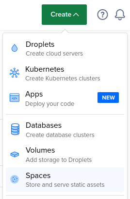
Then I set San Francisco as the datacenter region because I already had other spaces there.
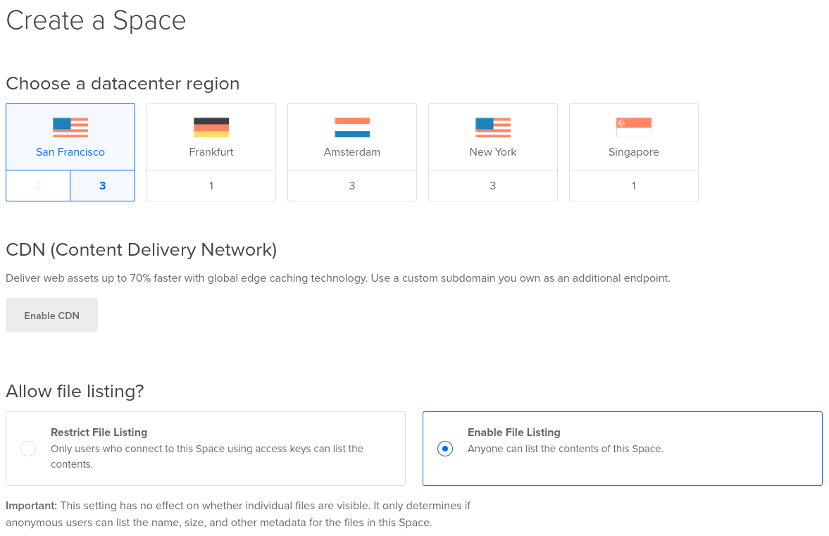
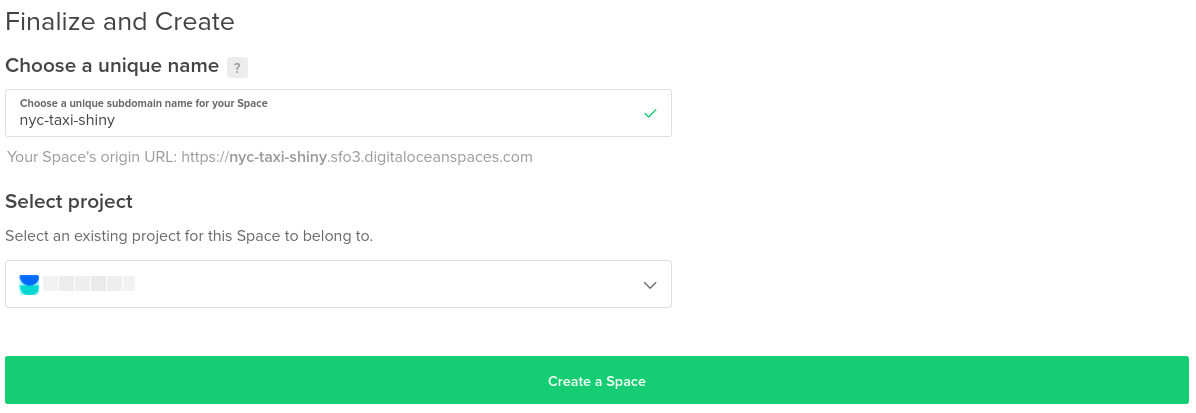
This creates a fully-managed S3 bucket so you do not have to thing a ton about the underlying set-up or configuration.
At the time on writing, I was able to add unlimited S3 buckets up to 250GB for $5/month. If you don’t already have a DigitalOcean account, by using this link you’ll start with $100 in credits with a 2 months limit. This is enough for 1440 hours of computing on a machine with 4 GB memory and 2 dedicated CPUs and additional hours to experiment with 1 GB memory machines.
Right away, the bucket has launched and if we listed it as private or if we are going to write to it, we are going to need a key in order to read or write.

I already had a previous bucket with the data that I’m going to read for the Shiny example. The bucket just created will be used to store summaries of the data read by the app.

If you are going to need more buckets, it would be convenient to create those from RStudio (local or cloud) by using analogsea.
analogsea::space_create(
 name = "myspace",
 spaces_region = "sfo2",
 spaces_key = Sys.getenv("spaces_nyc_taxi_key"),
 spaces_secret = Sys.getenv("spaces_nyc_taxi_key")
)
Creating an RStudio Server droplet
To speed thingsup, I shall create a droplet (i.e. a virtual machine) and write and run my Shiny app from there, on the same network as the S3 bucket.
I can create this from the website:
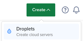


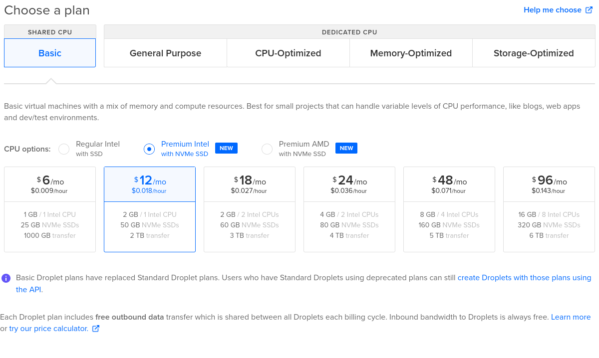


Or I can create this by using analogsea, where I ended up creating a droplet with 4GB in RAM.
library(analogsea)

# sizes()

droplet <- droplet_create(
  name = "shiny-post",
  size = "c2-2vcpu-4gb",
  region = "sfo3",
  image = "rstudio-20-04"
)
Now I can connect via SSH to add a non-root user (or I won’t be able to use RStudio Server from the browser), or I can do that from Rstudio Desktop.
droplet_ip(droplet)

set.seed(1234)
pass <- create_password()
ubuntu_create_user(droplet, "pacha", pass)
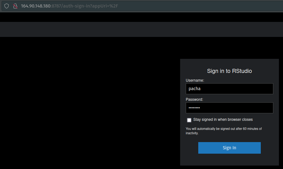
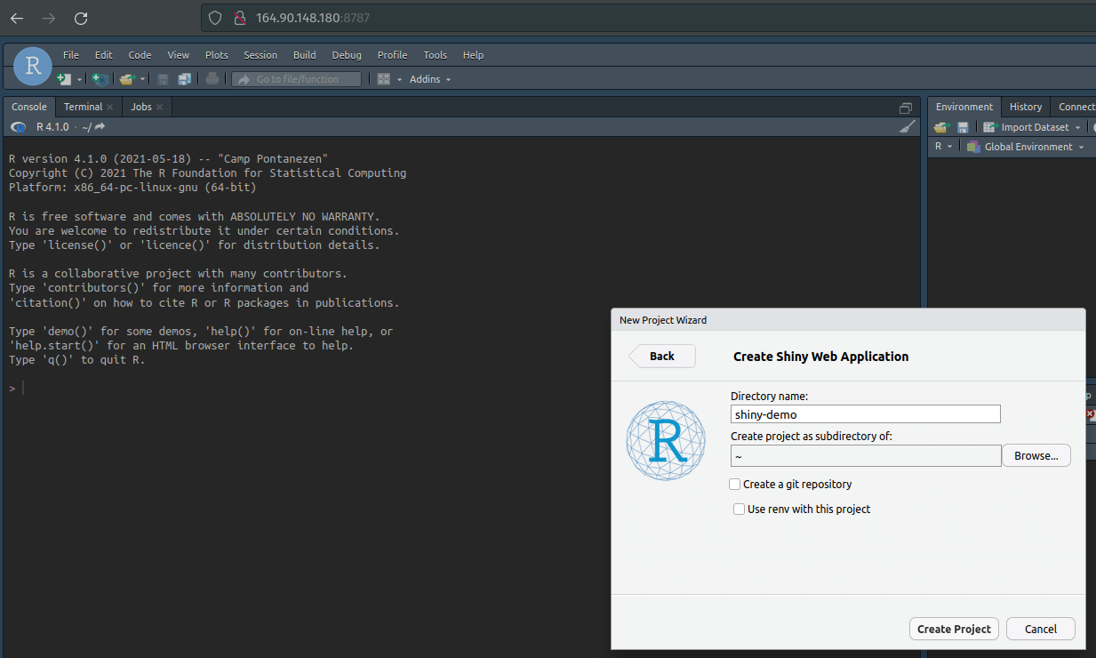
Now I can go to the IP obtained in the previous step on port 8787 (i.e. 164.90.148.180:8787) where I can use the user “pacha” and the pass created with analogsea to access and create a Shiny App project.
Connecting to the S3 bucket
I can minimally tweak the Old Faithful Geyser Data app to show how to read data in Parquet format with Apache Arrow that’s stored in the S3 bucket. We don’t need credentials to read from the S3 bucket nyc-taxi since it’s publicly listed.
library(shiny)
library(arrow)
library(dplyr)
library(ggplot2)

nyc_taxi <- S3FileSystem$create(
    anonymous = TRUE,
    scheme = "https",
    endpoint_override = "sfo3.digitaloceanspaces.com"
)

# Define UI for application that draws a histogram
ui <- fluidPage(

    # Application title
    titlePanel("NYC Taxi Data"),

    # Sidebar with a slider input for number of bins
    sidebarLayout(
        sidebarPanel(
            sliderInput("year", "Year:",
                        min = 2009, max = 2019, value = 2009),
            sliderInput("month", "Month:",
                        min = 1, max = 12, value = 1),
        ),

        # Show a plot of the generated distribution
        mainPanel(
            plotOutput("distPlot")
        )
    )
)

# Define server logic required to draw a histogram
server <- function(input, output) {

    output$distPlot <- renderPlot({
        y <- input$year
        m <- stringr::str_pad(input$month, 2, "left", "0")
        finp <- glue::glue("nyc-taxi/{y}/{m}/data.parquet")
        # read and count travels per day
        df <- read_parquet(nyc_taxi$path(finp))
        df <- df %>%
            as_tibble() %>%
            mutate(date = as.Date(pickup_at)) %>%
            group_by(date) %>%
            count()

        # draw the histogram
        ggplot(df) +
            geom_col(aes(x = date, y = n)) +
            labs(title = glue::glue("Travels per day {y}-{m}"))
    })
}

# Run the application
shinyApp(ui = ui, server = server)
This can be edited and run from the virtual machine!
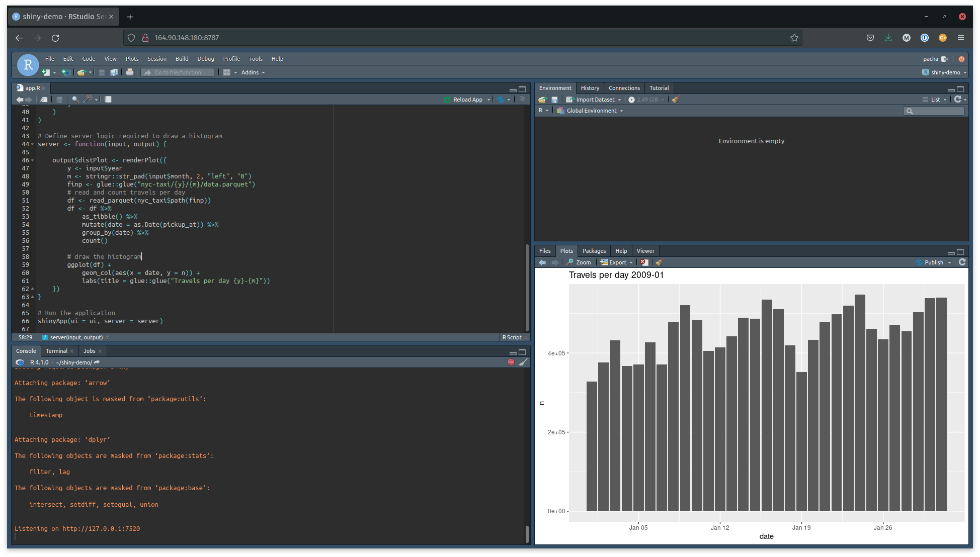
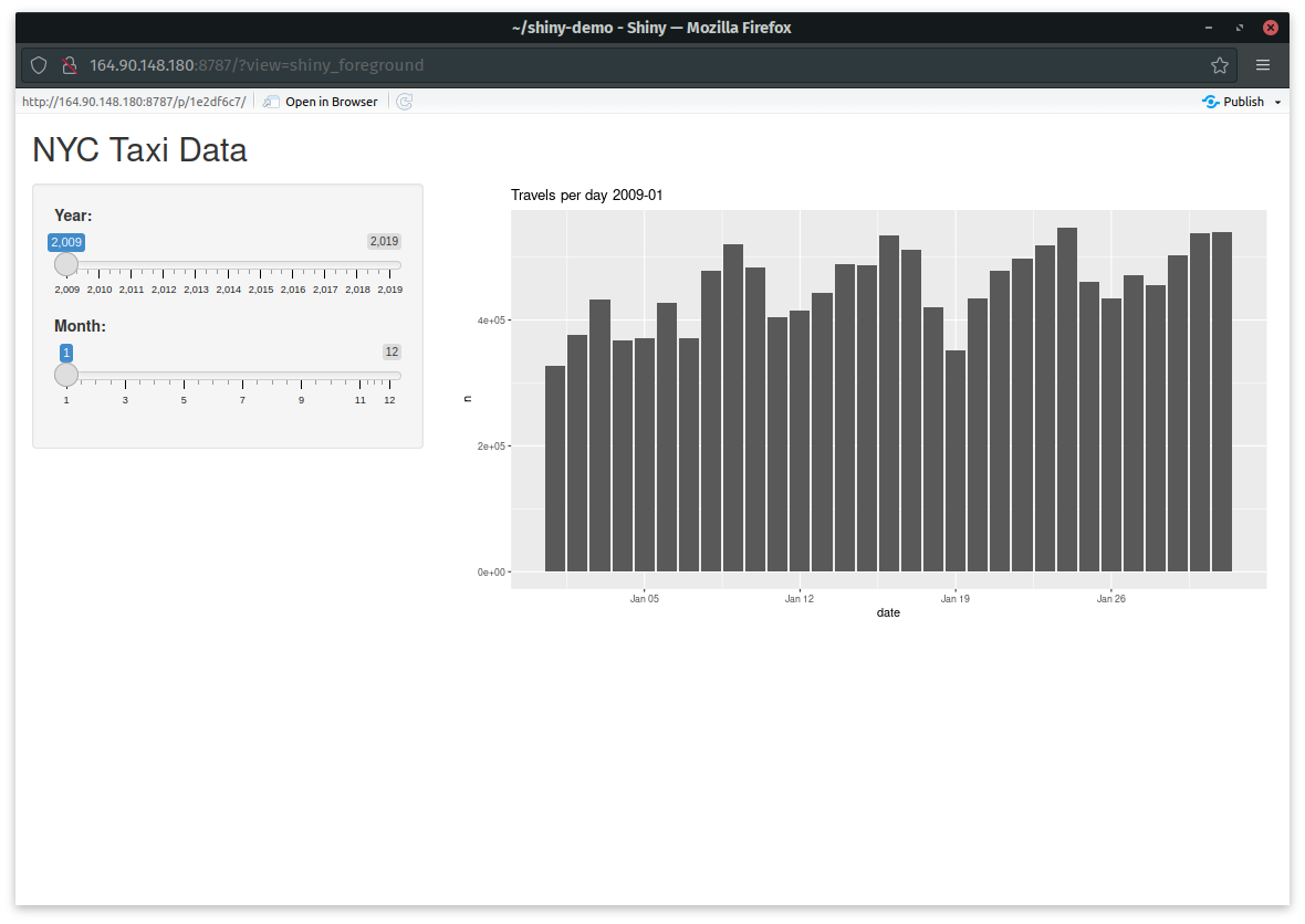
The biggest problem with this app is that it’s too slow. We could store the summary to avoid reading a table of 14,000,000 x 18 to create a summary of 30 x 2 each time.
One option is to write to the server and also write to the S3 bucket to create backups.
library(shiny)
library(arrow)
library(dplyr)
library(ggplot2)

nyc_taxi <- S3FileSystem$create(
    anonymous = TRUE,
    scheme = "https",
    endpoint_override = "sfo3.digitaloceanspaces.com"
)

nyc_taxi_shiny <- S3FileSystem$create(
    anonymous = FALSE,
    access_key = Sys.getenv("spaces_nyc_taxi_key"),
    secret_key = Sys.getenv("spaces_nyc_taxi_secret"),
    scheme = "https",
    endpoint_override = "sfo3.digitaloceanspaces.com"
)

# Define UI for application that draws a histogram
ui <- fluidPage(

    # Application title
    titlePanel("NYC Taxi Data"),

    # Sidebar with a slider input for number of bins
    sidebarLayout(
        sidebarPanel(
            sliderInput("year", "Year:",
                        min = 2009, max = 2019, value = 2009),
            sliderInput("month", "Month:",
                        min = 1, max = 12, value = 1),
        ),

        # Show a plot of the generated distribution
        mainPanel(
            plotOutput("distPlot")
        )
    )
)

# Define server logic required to draw a histogram
server <- function(input, output) {

    output$distPlot <- renderPlot({
        y <- input$year
        m <- stringr::str_pad(input$month, 2, "left", "0")
        finp <- glue::glue("nyc-taxi/{y}/{m}/data.parquet")
        fout <- glue::glue("nyc-taxi-shiny/{y}/{m}")
        finp2 <- glue::glue("nyc-taxi-shiny/{y}/{m}/part-0.parquet")
        if (!file.exists(fout)) {
            # read and count travels per day
            df <- read_parquet(nyc_taxi$path(finp))
            df <- df %>%
                as_tibble() %>%
                mutate(date = as.Date(pickup_at)) %>%
                group_by(date) %>%
                count()

            write_dataset(df %>% ungroup(), fout)
            arrow::copy_files(fout, nyc_taxi_shiny$path(fout))
        } else {
            df <- read_parquet(nyc_taxi_shiny$path(finp2))
        }
        # draw the histogram
        ggplot(df) +
            geom_col(aes(x = date, y = n)) +
            labs(title = glue::glue("Travels per day {y}-{m}"))
    })
}

# Run the application
shinyApp(ui = ui, server = server)
Of course, this is not the only way to do this. In another post about Apache Arrow I copied a subset of the raw data to my laptop to conduct a test.
Moving from SQL to Arrow
For more complicated projects, it might be better to think about an API to serve the data. This is exactly how Open Trade Statistics works. This project used PostgreSQL until recently, when I moved to Apache Arrow for easier data updates. I keep an S3 bucket that I copy to same server where the data API runs and then a second server runs the Shiny app. All of this also on DigitalOcean.
The reason for the update is that I had a ~50 GB table, where I had to upload new rows and update indexes. With Arrow I just delete the respective year/country to update and the index is the directory tree itself. Another Arrow magic is that you can run rclone sync back and forth and it automatically updates, say, 100 MB of 50 GB in data in a few seconds. With PostgreSQL the update is not that easy but the ideal tool depends on the project and a series of technical considerations too broad to cover in one post.
Secure HTTPS and SSH
This is something to consider to secure your shiny app:
- Serve your app over HTTPS: https://www.digitalocean.com/community/tutorials/how-to-secure-nginx-with-let-s-encrypt-on-ubuntu-18-04
- Use SSH keys instead of typed passwords to enter your server via SSH: https://www.digitalocean.com/docs/droplets/how-to/add-ssh-keys/
- Configure an application such as Google Authenticator to provide a dynamic additional password for SSH access: https://www.digitalocean.com/community/tutorials/how-to-protect-ssh-with-two-factor-authentication
You might be interested in looking at the NGINX configuration files that I used for Open Trade Statistics before enabling HTTPS with Let’s Encrypt.
Shameless self-promotion: If you liked this post, I am an Applied Statistician with years of experience in R, Shiny, APIs, SQL and finance. If you think I can be a valuable addition for your team, I’m happy to read from you and provide more details. My email is mavargas 11 [ at ] uc dot cl or send me a tweet to pachadotdev.