analogsea: Using Arrow, S3 and DigitalOcean for efficient model fitting in RStudio

How to fit models by using the cloud with a minimal data transfer to your laptop.

Introduction

This tutorial explains how to use arrow with analogsea to take fully advantage from S3 filesystems and parallel computing.

Analogsea is a community project created by and for statisticians from the R community: Scott Chamberlain, Hadley Wickham, Winston Chang, Bob Rudis, Bryce Mecum, and yours truly. This package provides an interface to DigitalOcean, a cloud service such as AWS, Linode and others, for R users.

Even when DigitalOcean provides an API, computing across clusters composed by virtual servers is not straightforward, since vanilla Ubuntu servers (‘droplets’ in DO jargon) require additional configurations to install R itself and numerical libraries such as OpenBLAS.

The configuration problem is largely reduced with the RStudio image from DigitalOcean Marketplace. In the last two years, the RStudio image for the Marketplace has provided a multipurpose image with out-of-box Shiny Server and common R packages such as the Tidvyerse and common SQL connectors, and now a configuration to use Arrow with S3 filesystems.

Just as an example, the Catholic University of Chile, the best university of Chile and one of the few in Latin America with excellent research metrics, uses Arrow and the mentioned RStudio image to offer a Covid Dashboard for Chile.

This tutorial is somewhat based in a blog post by Dr. Andrew Heiss, while most of the steps are simplified here thanks to newer software developments.

NYC Taxi dataset

You can have a look at the NYC Taxi dataset, which is stored in DigitalOcean Spaces with S3 compatible features. You can copy and explore the data locally like this.

library(arrow)

space <- S3FileSystem$create(
  anonymous = TRUE,
  scheme = "https",
  endpoint_override = "sfo3.digitaloceanspaces.com"
)

# just 2009/01 for a quick exploration
try(dir.create("~/nyc-taxi/2009/01", recursive = T))
arrow::copy_files(space$path("nyc-taxi/2009/01"), "~/nyc-taxi/2009/01")

d <- open_dataset(
  "~/nyc-taxi",
  partitioning = c("year", "month")
)

d

## FileSystemDataset with 1 Parquet file
## vendor_id: string
## pickup_at: timestamp[us]
## dropoff_at: timestamp[us]
## passenger_count: int8
## trip_distance: float
## pickup_longitude: float
## pickup_latitude: float
## rate_code_id: null
## store_and_fwd_flag: string
## dropoff_longitude: float
## dropoff_latitude: float
## payment_type: string
## fare_amount: float
## extra: float
## mta_tax: float
## tip_amount: float
## tolls_amount: float
## total_amount: float
## year: int32
## month: int32
## 
## See $metadata for additional Schema metadata

One interesting exercise is to explore how trip distance and total amount are related. You can fit a regression to do that! But you should explore the data first, and a good way to do so is to visualize how the observations are distributed.

library(dplyr)

dreg <- d %>% 
  select(trip_distance, total_amount) %>% 
  collect()

dreg

## # A tibble: 14,092,413 x 2
##    trip_distance total_amount
##            <dbl>        <dbl>
##  1         2.63          9.40
##  2         4.55         14.6 
##  3        10.4          28.4 
##  4         5            18.5 
##  5         0.400         3.70
##  6         1.20          6.60
##  7         0.400         6.70
##  8         1.72          6.60
##  9         1.60         10   
## 10         0.700         5.90
## # … with 14,092,403 more rows

As this is a ~14 million rows for a single month, it will be hard to plot without at least some aggregation. There are repeated rows so you can count to get the frequencies for the pairs (distance, amount), and even round the numbers before doing aggregation since the idea is to explore if there’s a trend.

dplot <- dreg %>% 
  mutate_if(is.numeric, function(x) round(x,0)) %>% 
  group_by(trip_distance, total_amount) %>% 
  count()

dplot

## # A tibble: 4,070 x 3
## # Groups:   trip_distance, total_amount [4,070]
##    trip_distance total_amount      n
##            <dbl>        <dbl>  <int>
##  1             0            2  39663
##  2             0            3 181606
##  3             0            4 421546
##  4             0            5 165490
##  5             0            6  63610
##  6             0            7  26822
##  7             0            8  20584
##  8             0            9  13889
##  9             0           10  12073
## 10             0           11   8271
## # … with 4,060 more rows

There is not an obvious trend in this data, but it’s still possible to obtain a trend line.

library(ggplot2)

ggplot(dplot, aes(x = trip_distance, y = total_amount, alpha = log(n))) +
  geom_jitter() +
  labs(title = "Exploring distance versus total amount")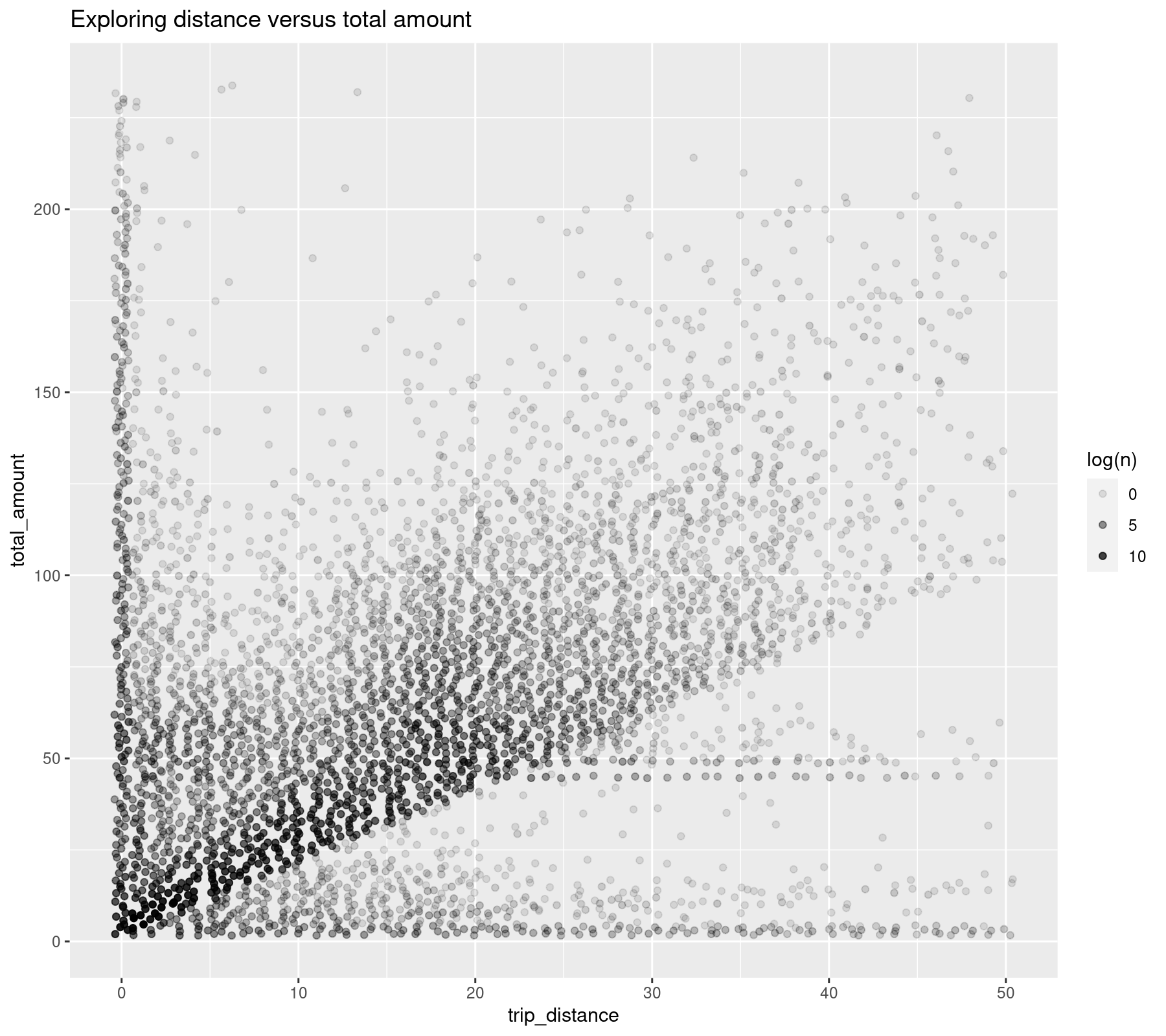

You can fit a model with Gaussian errors such as the next model with intercept.

summary(lm(total_amount ~ trip_distance, data = dreg))

## 
## Call:
## lm(formula = total_amount ~ trip_distance, data = dreg)
## 
## Residuals:
##      Min       1Q   Median       3Q      Max 
## -122.736   -1.242   -0.542    0.509  228.125 
## 
## Coefficients:
##                Estimate Std. Error t value Pr(>|t|)    
## (Intercept)   4.0253576  0.0013786    2920   <2e-16 ***
## trip_distance 2.4388382  0.0003532    6905   <2e-16 ***
## ---
## Signif. codes:  0 '***' 0.001 '**' 0.01 '*' 0.05 '.' 0.1 ' ' 1
## 
## Residual standard error: 3.909 on 14092411 degrees of freedom
## Multiple R-squared:  0.7718, Adjusted R-squared:  0.7718 
## F-statistic: 4.767e+07 on 1 and 14092411 DF,  p-value: < 2.2e-16

Fitting models in the cloud

Let’s say we are interested in fitting one model per month and then average the obtain coefficients to smooth a potential seasonal effect (e.g. such as holidays, Christmas, etc).

To do this you can create 1,2,…,N droplets and assign different months to each droplet and read the data from S3, to then get the regression results to your laptop.

You can start by loading the analogsea package and create two droplets that already include arrow. The next code assumes that you already registered your SSH key at digitalocean.com.

library(analogsea)

s <- "c-8" # 4 dedicated CPUs + 8GB memory, run sizes()
droplet1 <- droplet_create("RDemo1", region = "sfo3", size = s, 
                           image = "rstudio-20-04", wait = F)
droplet2 <- droplet_create("RDemo2", region = "sfo3", size = s, 
                           image = "rstudio-20-04", wait = T)

What if you need to install additional R packages in the droplets? Well, you can control that remotely after updating the droplet status and install, for example, eflm to speed-up the regressions.

droplet1 <- droplet(droplet1$id)
droplet2 <- droplet(droplet2$id)

install_r_package(droplet1, "eflm")
install_r_package(droplet2, "eflm")

Before proceeding, you need the droplet’s IPs to create a cluster that will use each droplet as a CPU core from your laptop.

ip1 <- droplet(droplet1$id)$networks$v4[[2]]$ip_address
ip2 <- droplet(droplet2$id)$networks$v4[[2]]$ip_address
ips <- c(ip1, ip2)

Now you can create a cluster, and you need to specify which SSH key to use.

library(future)

ssh_private_key_file <- "~/.ssh/id_rsa"

cl <- makeClusterPSOCK(
  ips,
  user = "root",
  rshopts = c(
    "-o", "StrictHostKeyChecking=no",
    "-o", "IdentitiesOnly=yes",
    "-i", ssh_private_key_file
  ),
  dryrun = FALSE
)

The next step is to create a working plan (i.e. 1 droplet = 1 ‘CPU core’) which allows to run processes in parallel and a function to specify which data to read and how to fit the models in the droplets.

plan(cluster, workers = cl)

fit_model <- function(y, m) {
  message(paste(y,m))

  suppressMessages(library(arrow))
  suppressMessages(library(dplyr))

  space <- S3FileSystem$create(
    anonymous = TRUE,
    scheme = "https",
    endpoint_override = "sfo3.digitaloceanspaces.com"
  )

  d <- open_dataset(
    space$path("nyc-taxi"),
    partitioning = c("year", "month")
  )

  d <- d %>%
    filter(year == y, month == m) %>%
    select(total_amount, trip_distance) %>%
    collect()

  fit <- try(eflm::elm(total_amount ~ trip_distance, data = d, model = F))
  if (class(fit) == "lm") fit <- fit$coefficients
  rm(d); gc()
  return(fit)
}

The fit_model function is a function that you should iterate over months and years. The furrr package is very efficient for these tasks and works well with the working plan defined previously, and the iteration can be run in a very similar way to purrr.

library(furrr)

fitted_models <- future_map2(
  c(rep(2009, 12),rep(2010, 12)), rep(1:12,2), ~fit_model(.x, .y))
  
fitted_models[[1]]

# (Intercept) trip_distance 
#    4.025358      2.438838

In the previous code, even when the iteration was made with two years there are some clear efficiencies. On the one hand, the data is read from S3 without leaving DigitalOcean network, and any problem with home connections is therefore eliminated because you only have to upload a text with the function to the droplets and then you get the estimated coefficients without moving gigabytes of data to your laptop. On the other, and the computation is run in parallel so I could create more droplets to reduce the reading and fitting times even more.

Using the results from the cloud

If you want to average the estimated coefficients, you need to subset and discard the unusable months.

intercept <- c()
slope <- c()

for (i in seq_along(fitted_models)) {
  intercept[i] <- ifelse(is.numeric(fitted_models[[i]]),
                         fitted_models[[i]][1], NA)
  slope[i] <- ifelse(is.numeric(fitted_models[[i]]),
                           fitted_models[[i]][2], NA)
}

avg_coefficients <- c(mean(intercept, na.rm = T), mean(slope, na.rm = T))
names(avg_coefficients) <- c("intercept", "slope")

avg_coefficients

# intercept     slope 
#  4.406586  2.533299

Now you can say that, on average, if you travelled 5 miles by taxi, you’d expect to pay 4.4 + 2.5 x 5 ~= 17 USD, which is just an estimate depending on traffic conditions, finding many red lights, etc.

Don’t forget to delete the droplets when you are done using them.

droplet_delete(droplet1)
droplet_delete(droplet2)

Final remarks

Arrow and S3 provide a powerful combination for big data analysis. You can even create a droplet to control other droplets if you feat that your internet connection is not that good like to transfer complete regression summaries.

Think about the possibility of fitting many other models: generalized linear models, random forest, non-linear regression, posterior bootstrap, or basically any output that R understands.