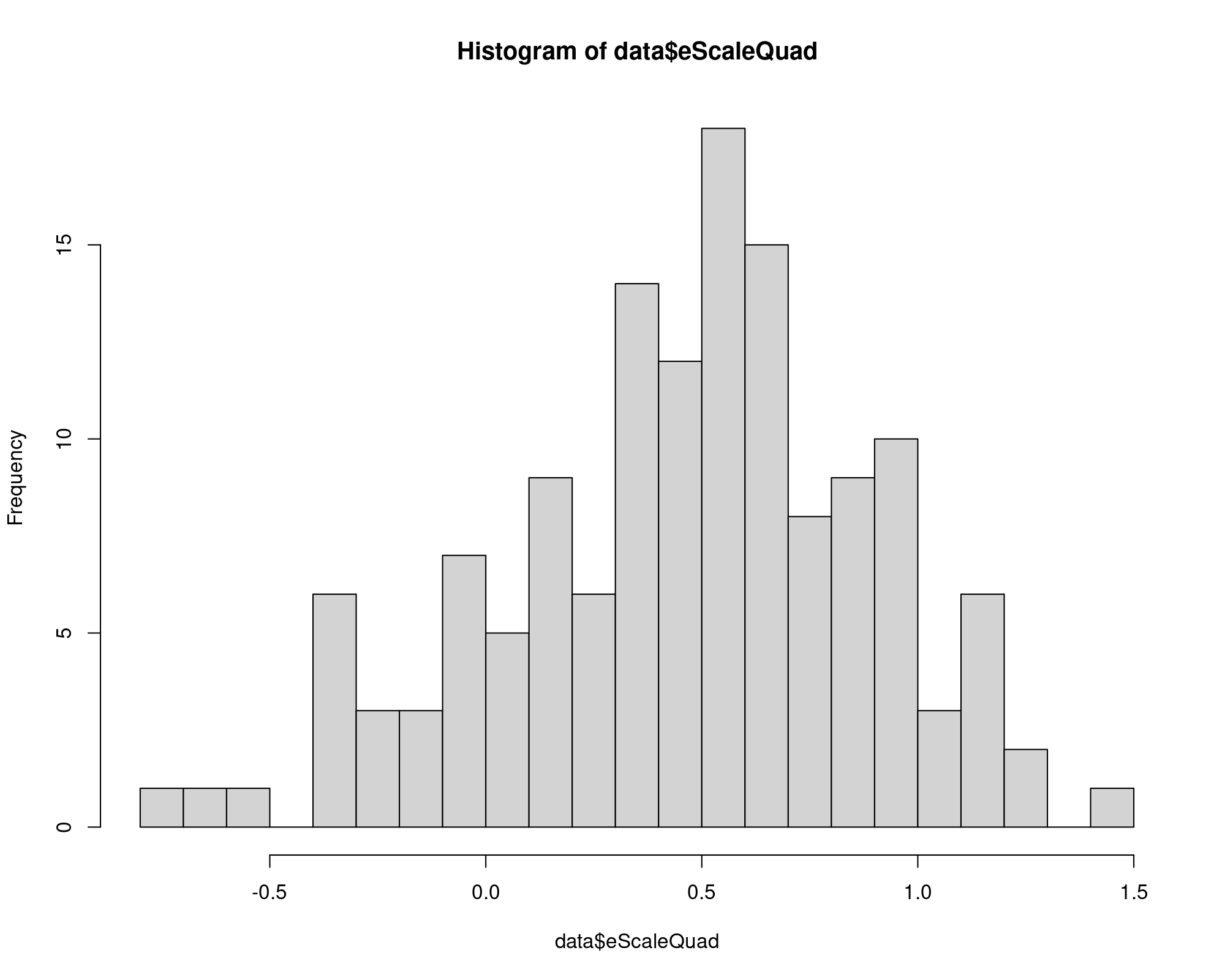
data$eScaleQuad = data$eCapQuad + data$eCapTL + data$eCapTL
sum(data$eScaleQuad < 0)
[1] 22
summary(data$eScaleQuad)
Min. 1st Qu. Median Mean 3rd Qu. Max.
-0.7436 0.1755 0.5162 0.4576 0.7239 1.4552
hist(data$eScaleQuad, breaks=20)Microeconomic Theory and Linear Regression
Linear models and models comparison to estimate apples production.
Introduction
This is a summary of a very old collection of materials that I used as teaching assistant (before 2017).
Among those materials I found some class notes from Arne Henningsen, the author of micEcon R package.
I’ll use that package and some others to show some concepts from Microeconomic Theory.
Packages installation:
# install.packages(c("micEcon","lmtest","bbmle","miscTools"))
library(micEcon)
library(lmtest)
library(stats4) #this is a base package so don't install this!
library(bbmle)
library(miscTools)
From package’s help: “The appleProdFr86 data frame includes cross-sectional production data of 140 French apple producers from the year 1986. These data have been extracted from a panel data set that was used in Ivaldi et al. (1996).”
This data frame contains the following columns:
| Variable | Description |
|---|---|
| vCap | costs of capital (including land) |
| vLab | costs of labour (including remuneration of unpaid family labour) |
| vMat | costs of intermediate materials (e.g. seedlings, fertilizer, pesticides, fuel) |
| qApples | quantity index of produced apples |
| qOtherOut | quantity index of all other outputs |
| qOut | quantity index of all outputs (not in the original data set, calculated as \(580,000 \times (qApples + qOtherOut)\)) |
| pCap | price index of capital goods |
| pLab | price index of labour |
| pMat | price index of materials |
| pOut | price index of the aggregate output (not in the original data set, artificially generated) |
| adv | dummy variable indicating the use of an advisory service (not in the original data set, artificially generated) |
Now I’ll examine appleProdFr86 dataset:
data("appleProdFr86", package = "micEcon")
data = appleProdFr86
rm(appleProdFr86)
str(data)

'data.frame':   140 obs. of  11 variables:
 $ vCap     : int  219183 130572 81301 34007 38702 122400 89061 92134 65779 94047 ...
 $ vLab     : int  323991 187956 134147 105794 83717 523842 168140 204859 180598 142240 ...
 $ vMat     : int  303155 262017 90592 59833 104159 577468 343768 126547 190622 82357 ...
 $ qApples  : num  1.392 0.864 3.317 0.438 1.831 ...
 $ qOtherOut: num  0.977 1.072 0.405 0.436 0.015 ...
 $ qOut     : num  1374064 1122979 2158518 507389 1070816 ...
 $ pCap     : num  2.608 3.292 2.194 1.602 0.866 ...
 $ pLab     : num  0.9 0.753 0.956 1.268 0.938 ...
 $ pMat     : num  8.89 6.42 3.74 3.17 7.22 ...
 $ pOut     : num  0.66 0.716 0.937 0.597 0.825 ...
 $ adv      : num  0 0 1 1 1 1 1 0 0 0 ...
Linear Production Function
A linear production function is of the form: \[y = \beta_0 + \sum_i \beta_i x_i\] And from that I’ll estimate the function coefficients and a prediction of the output.
The dataset does not provide units of capital, labour or materials, but it provides information about costs and price index. Then I create the variables for the units from that:
data$qCap = data$vCap/data$pCap
data$qLab = data$vLab/data$pLab
data$qMat = data$vMat/data$pMat
Let \(\rho\) be the linear correlation coefficient. The hypothesis testing of Linear Correlation Between Variables is: \[H_0:\: \rho = 0\\ H_1:\: \rho\neq 0\]
To test this I’ll use the statistic: \[ t = r \sqrt{\frac{n-2}{1-r^2}} \] that follows a t-Student distribution with \(n-2\) degrees of freedom.
And the correlation test for each input is:
cor.test(data$qOut, data$qCap, alternative="greater")


    Pearson's product-moment correlation

data:  data$qOut and data$qCap
t = 8.7546, df = 138, p-value = 3.248e-15
alternative hypothesis: true correlation is greater than 0
95 percent confidence interval:
 0.4996247 1.0000000
sample estimates:
      cor
0.5975547

cor.test(data$qOut, data$qLab, alternative="greater")

    Pearson's product-moment correlation

data:  data$qOut and data$qLab
t = 20.203, df = 138, p-value < 2.2e-16
alternative hypothesis: true correlation is greater than 0
95 percent confidence interval:
 0.8243685 1.0000000
sample estimates:
      cor
0.8644853

cor.test(data$qOut, data$qMat, alternative="greater")


    Pearson's product-moment correlation

data:  data$qOut and data$qMat
t = 15.792, df = 138, p-value < 2.2e-16
alternative hypothesis: true correlation is greater than 0
95 percent confidence interval:
 0.7463428 1.0000000
sample estimates:
      cor
0.8023509
With the units of input I write the production function and estimate its coefficients:
prodLin = lm(qOut ~ qCap + qLab + qMat, data = data)
data$qOutLin = fitted(prodLin)
summary(prodLin)

Call:
lm(formula = qOut ~ qCap + qLab + qMat, data = data)

Residuals:
     Min       1Q   Median       3Q      Max
-3888955  -773002    86119   769073  7091521

Coefficients:
              Estimate Std. Error t value Pr(>|t|)
(Intercept) -1.616e+06  2.318e+05  -6.972 1.23e-10 ***
qCap         1.788e+00  1.995e+00   0.896    0.372
qLab         1.183e+01  1.272e+00   9.300 3.15e-16 ***
qMat         4.667e+01  1.123e+01   4.154 5.74e-05 ***
---
Signif. codes:  0 '***' 0.001 '**' 0.01 '*' 0.05 '.' 0.1 ' ' 1

Residual standard error: 1541000 on 136 degrees of freedom
Multiple R-squared:  0.7868,    Adjusted R-squared:  0.7821
F-statistic: 167.3 on 3 and 136 DF,  p-value: < 2.2e-16
I can also use Log-Likelihood to obtain the estimates:
LogLikelihood = function(beta0, betacap, betalab, betamat, mu, sigma) {
  R = data$qOut - (beta0 + betacap*data$qCap + betalab*data$qLab + betamat*data$qMat)
  R = suppressWarnings(dnorm(R, mu, sigma, log = TRUE))
  -sum(R)
}

prodLin2 = mle2(LogLikelihood, start = list(beta0 = 0, betacap = 10, betalab = 20, betamat = 30,
                                            mu = 0, sigma=1), control = list(maxit= 10000))
summary(prodLin)

Call:
lm(formula = qOut ~ qCap + qLab + qMat, data = data)

Residuals:
     Min       1Q   Median       3Q      Max
-3888955  -773002    86119   769073  7091521

Coefficients:
              Estimate Std. Error t value Pr(>|t|)
(Intercept) -1.616e+06  2.318e+05  -6.972 1.23e-10 ***
qCap         1.788e+00  1.995e+00   0.896    0.372
qLab         1.183e+01  1.272e+00   9.300 3.15e-16 ***
qMat         4.667e+01  1.123e+01   4.154 5.74e-05 ***
---
Signif. codes:  0 '***' 0.001 '**' 0.01 '*' 0.05 '.' 0.1 ' ' 1

Residual standard error: 1541000 on 136 degrees of freedom
Multiple R-squared:  0.7868,    Adjusted R-squared:  0.7821
F-statistic: 167.3 on 3 and 136 DF,  p-value: < 2.2e-16
Quadratic Production Function
A quadratic production function is of the form: \[y = \beta_0 + \sum_i \beta_i x_i + \frac{1}{2} \sum_i \sum_j \beta_{ij} x_i x_j\] And from that I’ll estimate the function coefficients and a prediction of the output.
With the arrangements made for the linear case now I have it ready to obtain the coefficients and the predicted output:
prodQuad = lm(qOut ~ qCap + qLab + qMat + I(0.5*qCap^2) + I(0.5*qLab^2) + I(0.5*qMat^2)
               + I(qCap*qLab) + I(qCap*qMat) + I(qLab*qMat), data = data)
data$qOutQuad = fitted(prodQuad)
summary(prodQuad)

Call:
lm(formula = qOut ~ qCap + qLab + qMat + I(0.5 * qCap^2) + I(0.5 *
    qLab^2) + I(0.5 * qMat^2) + I(qCap * qLab) + I(qCap * qMat) +
    I(qLab * qMat), data = data)

Residuals:
     Min       1Q   Median       3Q      Max
-3928802  -695518  -186123   545509  4474143

Coefficients:
                  Estimate Std. Error t value Pr(>|t|)
(Intercept)     -2.911e+05  3.615e+05  -0.805 0.422072
qCap             5.270e+00  4.403e+00   1.197 0.233532
qLab             6.077e+00  3.185e+00   1.908 0.058581 .
qMat             1.430e+01  2.406e+01   0.595 0.553168
I(0.5 * qCap^2)  5.032e-05  3.699e-05   1.360 0.176039
I(0.5 * qLab^2) -3.084e-05  2.081e-05  -1.482 0.140671
I(0.5 * qMat^2) -1.896e-03  8.951e-04  -2.118 0.036106 *
I(qCap * qLab)  -3.097e-05  1.498e-05  -2.067 0.040763 *
I(qCap * qMat)  -4.160e-05  1.474e-04  -0.282 0.778206
I(qLab * qMat)   4.011e-04  1.112e-04   3.608 0.000439 ***
---
Signif. codes:  0 '***' 0.001 '**' 0.01 '*' 0.05 '.' 0.1 ' ' 1

Residual standard error: 1344000 on 130 degrees of freedom
Multiple R-squared:  0.8449,    Adjusted R-squared:  0.8342
F-statistic: 78.68 on 9 and 130 DF,  p-value: < 2.2e-16
Linear Specification vs Quadratic Specification
From the above, which of the models is better? Wald Test, Likelihood Ratio Test and ANOVA can help. In this case I’m working with nested models, because the Linear Specification is contained within the Quadratic Specification:
waldtest(prodLin, prodQuad)

Wald test

Model 1: qOut ~ qCap + qLab + qMat
Model 2: qOut ~ qCap + qLab + qMat + I(0.5 * qCap^2) + I(0.5 * qLab^2) +
    I(0.5 * qMat^2) + I(qCap * qLab) + I(qCap * qMat) + I(qLab *
    qMat)
  Res.Df Df      F    Pr(>F)
1    136
2    130  6 8.1133 1.869e-07 ***
---
Signif. codes:  0 '***' 0.001 '**' 0.01 '*' 0.05 '.' 0.1 ' ' 1

lrtest(prodLin, prodQuad)

Likelihood ratio test

Model 1: qOut ~ qCap + qLab + qMat
Model 2: qOut ~ qCap + qLab + qMat + I(0.5 * qCap^2) + I(0.5 * qLab^2) +
    I(0.5 * qMat^2) + I(qCap * qLab) + I(qCap * qMat) + I(qLab *
    qMat)
  #Df  LogLik Df  Chisq Pr(>Chisq)
1   5 -2191.3
2  11 -2169.1  6 44.529  5.806e-08 ***
---
Signif. codes:  0 '***' 0.001 '**' 0.01 '*' 0.05 '.' 0.1 ' ' 1

anova(prodLin, prodQuad, test = "F")

Analysis of Variance Table

Model 1: qOut ~ qCap + qLab + qMat
Model 2: qOut ~ qCap + qLab + qMat + I(0.5 * qCap^2) + I(0.5 * qLab^2) +
    I(0.5 * qMat^2) + I(qCap * qLab) + I(qCap * qMat) + I(qLab *
    qMat)
  Res.Df        RSS Df  Sum of Sq      F    Pr(>F)
1    136 3.2285e+14
2    130 2.3489e+14  6 8.7957e+13 8.1133 1.869e-07 ***
---
Signif. codes:  0 '***' 0.001 '**' 0.01 '*' 0.05 '.' 0.1 ' ' 1
From the results the Quadratic Specification should be preferred as the tests show that the additional variables do add information.
Cobb-Douglas Production Function
A Cobb-Douglas production function is of the form: \[y = A \prod_i x_i^{\beta_i} \] And from that I’ll estimate the function coefficients and a prediction of the output.
This function is not linear, so I need to convert the function before fitting: \[\ln(y) = \ln(A) + \sum_{i=1}^n \beta_i \ln(x_i)\]
With the arrangements made for the linear case now I have it ready to obtain the coefficients and the predicted output:
prodCD = lm(log(qOut) ~ log(qCap) + log(qLab) + log(qMat), data = data)
data$qOutCD = fitted(prodCD)
summary(prodCD)

Call:
lm(formula = log(qOut) ~ log(qCap) + log(qLab) + log(qMat), data = data)

Residuals:
     Min       1Q   Median       3Q      Max
-1.67239 -0.28024  0.00667  0.47834  1.30115

Coefficients:
            Estimate Std. Error t value Pr(>|t|)
(Intercept) -2.06377    1.31259  -1.572   0.1182
log(qCap)    0.16303    0.08721   1.869   0.0637 .
log(qLab)    0.67622    0.15430   4.383 2.33e-05 ***
log(qMat)    0.62720    0.12587   4.983 1.87e-06 ***
---
Signif. codes:  0 '***' 0.001 '**' 0.01 '*' 0.05 '.' 0.1 ' ' 1

Residual standard error: 0.656 on 136 degrees of freedom
Multiple R-squared:  0.5943,    Adjusted R-squared:  0.5854
F-statistic: 66.41 on 3 and 136 DF,  p-value: < 2.2e-16
Translog Production Function
A Translog production function is of the form: \[\ln y = \beta_0 + \sum_i \alpha_i \ln x_i + \frac{1}{2} \sum_i \sum_j \beta_{ij} \ln x_i \ln x_j\] And from that I’ll estimate the function coefficients and a prediction of the output.
With the arrangements made for the linear case now I have it ready to obtain the coefficients and the predicted output:
prodTL = lm(log(qOut) ~ log(qCap) + log(qLab) + log(qMat) + I(0.5*log(qCap)^2)
             + I(0.5*log(qLab)^2) + I(0.5*log(qMat)^2) + I(log(qCap)*log(qLab))
             + I(log(qCap)*log(qMat)) + I(log(qLab)*log(qMat)), data = data)
data$qOutTL = fitted(prodTL)
summary(prodTL)

Call:
lm(formula = log(qOut) ~ log(qCap) + log(qLab) + log(qMat) +
    I(0.5 * log(qCap)^2) + I(0.5 * log(qLab)^2) + I(0.5 * log(qMat)^2) +
    I(log(qCap) * log(qLab)) + I(log(qCap) * log(qMat)) + I(log(qLab) *
    log(qMat)), data = data)

Residuals:
     Min       1Q   Median       3Q      Max
-1.68015 -0.36688  0.05389  0.44125  1.26560

Coefficients:
                         Estimate Std. Error t value Pr(>|t|)
(Intercept)              -4.14581   21.35945  -0.194   0.8464
log(qCap)                -2.30683    2.28829  -1.008   0.3153
log(qLab)                 1.99328    4.56624   0.437   0.6632
log(qMat)                 2.23170    3.76334   0.593   0.5542
I(0.5 * log(qCap)^2)     -0.02573    0.20834  -0.124   0.9019
I(0.5 * log(qLab)^2)     -1.16364    0.67943  -1.713   0.0892 .
I(0.5 * log(qMat)^2)     -0.50368    0.43498  -1.158   0.2490
I(log(qCap) * log(qLab))  0.56194    0.29120   1.930   0.0558 .
I(log(qCap) * log(qMat)) -0.40996    0.23534  -1.742   0.0839 .
I(log(qLab) * log(qMat))  0.65793    0.42750   1.539   0.1262
---
Signif. codes:  0 '***' 0.001 '**' 0.01 '*' 0.05 '.' 0.1 ' ' 1

Residual standard error: 0.6412 on 130 degrees of freedom
Multiple R-squared:  0.6296,    Adjusted R-squared:  0.6039
F-statistic: 24.55 on 9 and 130 DF,  p-value: < 2.2e-16
Cobb-Douglas Specification vs Translog Specification
This is really similar to the comparison between Linear Specification and Quadratic Specification. In this case the models are nested too and the tests are:
waldtest(prodCD, prodTL)
lrtest(prodCD, prodTL)
anova(prodCD, prodTL, test = "F")

Wald test

Model 1: log(qOut) ~ log(qCap) + log(qLab) + log(qMat)
Model 2: log(qOut) ~ log(qCap) + log(qLab) + log(qMat) + I(0.5 * log(qCap)^2) +
    I(0.5 * log(qLab)^2) + I(0.5 * log(qMat)^2) + I(log(qCap) *
    log(qLab)) + I(log(qCap) * log(qMat)) + I(log(qLab) * log(qMat))
  Res.Df Df     F  Pr(>F)
1    136
2    130  6 2.062 0.06202 .
---
Signif. codes:  0 '***' 0.001 '**' 0.01 '*' 0.05 '.' 0.1 ' ' 1
From the results the Translog Specification should be preferred as the tests show that the additional variables do add information.
Quadratic Specification vs Translog Specification
The dependent variable is different (\(y\) versus \(\ln(y)\)) and I also cannot compare \(R^2\) or use tests for nested models.
What I can do is to calculate the hypothetical value of \(y\) by doing a logarithmic transformation to the Quadratic Specification and then I’ll obtain a comparable \(R^2\):
summary(prodTL)$r.squared; rSquared(log(data$qOut), log(data$qOut) - log(data$qOutQuad))

[1] 0.6295696

          [,1]
[1,] 0.5481309
\(\Longrightarrow\) the Translog Specification has a better fit on \(\ln(y)\).
Another option is to apply an exponential transformation to the Translog Specification and then I’ll obtain a comparable \(R^2\):
summary(prodQuad)$r.squared; rSquared(data$qOut, data$qOut - exp(data$qOutTL))

[1] 0.8448983

          [,1]
[1,] 0.7696638
\(\Longrightarrow\) the Quadratic Specification has a better fit on \(y\).
This table resumes this part of the analysis:
| Quadratic | Translog | |
|---|---|---|
| \(R^2\) on \(y\) | 0.85 | 0.77 |
| \(R^2\) on \(ln(y)\) | 0.55 | 0.63 |
Here I can compare \(R^2\) provided that the number of coefficients is the same. If the models had a different number of coefficients I should use \(\bar{R}^2\).
In any case, comparing \(R^2\) does not help to choose an Specification. An alternative is to verify the theoretical consistency of both Specifications.
Microeconomic Concepts
In this part I’ll use the Quadratic and Translog specifications given that those are the best fit models in the last exercises.
Plot of output versus predicted output after adjusting the scale:
data$qOutTL = exp(fitted(prodTL))
par(mfrow=c(1,2))
compPlot(data$qOut, data$qOutQuad, log = "xy", main = "Quadratic Specification")
compPlot(data$qOut, data$qOutTL, log = "xy", main = "Translog Specification")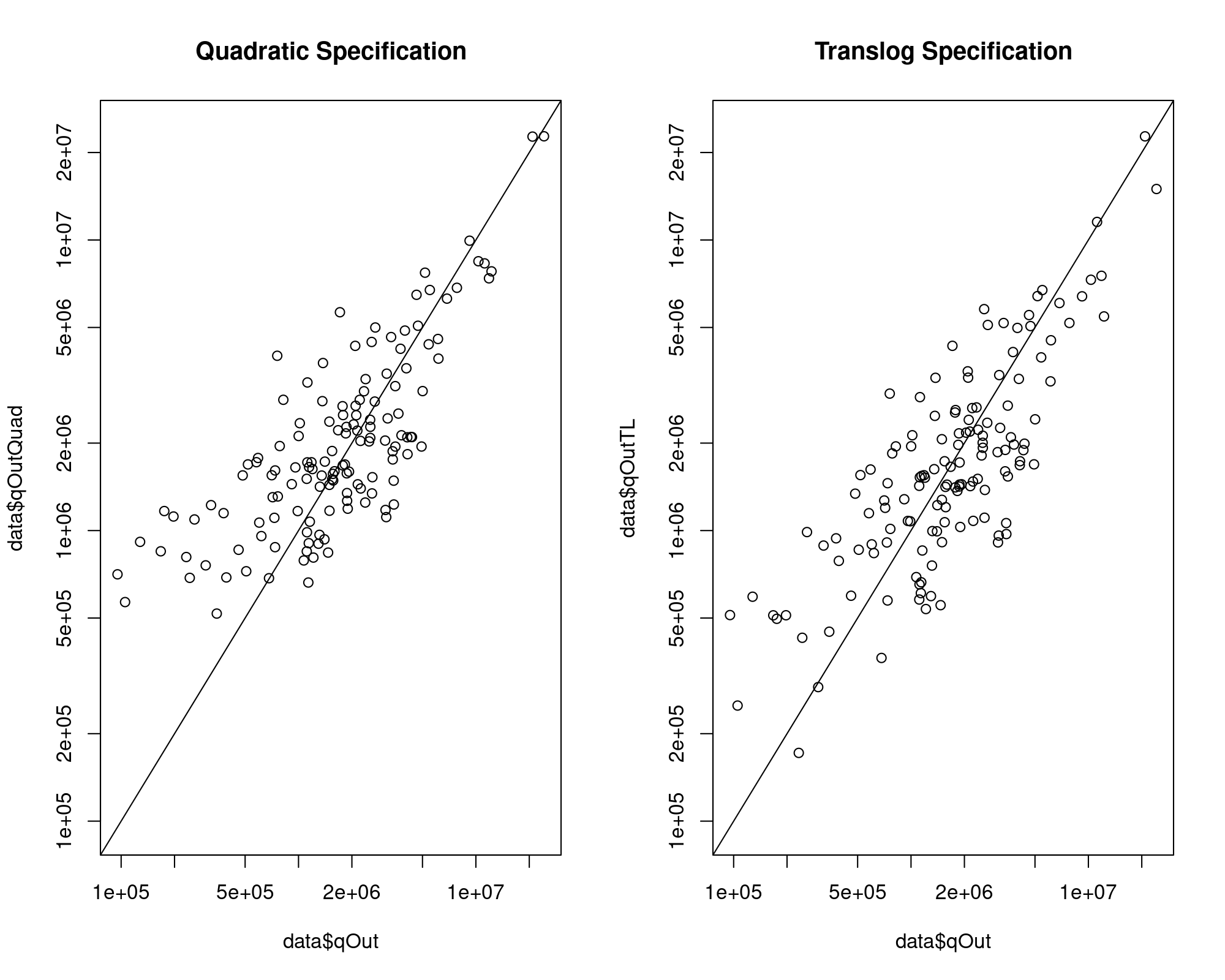
Provided that I have some negative coefficients both in Quadratic and Translog Specifications, there can be a negative predicted output:
sum(data$qOutQuad < 0); sum(data$qOutTL < 0)

[1] 0

[1] 0
That problem did not appear here.
Another problem that can appear from negative coefficients is a negative marginal effect after an increase in the inputs. Logically, an increase in the inputs should never decrease the output.
To check this I need the marginal productivity: \[MP_{i} = \frac{\partial y}{\partial x_i}\]
And the Product-Factor Elasticity: \[ \varepsilon_i = \frac{\partial \ln (y)}{\partial \ln(x_i)} \]
Another useful concept is Scale Elasticity: \[\varepsilon = \sum_{i=1}^n \varepsilon_i\]
In microeconomics, the concept of monotonicity refers to the fact that an increase in the inputs does not decreases the output. Then, an observation that does not violate monotonicity condition is an observation such that any of its calculated marginal productivities can at least be zero.
In the case of a Translog Specification the Product-Factor elasticity can be written as: \[ \varepsilon_i = \beta_i + \sum_{j=1}^n \beta_{ij} \ln(x_j) \]
Also keep in mind this about the Translog Specification: \[ \frac{\partial \ln(y)}{\partial \ln(x_i)} = \frac{\Delta y}{y} \frac{x_i}{\Delta x_i} \: \Longrightarrow \: MP_i = \frac{\partial y}{\partial x_i} = \frac{y}{x_i} \frac{\partial \ln(y)}{\partial \ln(x_i)} = \frac{y}{x_i}\varepsilon_i \]
So I’ll start with the Product-Factor Elasticity for the Translog Specification:
b1  = coef(prodTL)["log(qCap)"]
b2  = coef(prodTL)["log(qLab)"]
b3  = coef(prodTL)["log(qMat)"]
b11 = coef(prodTL)["I(0.5 * log(qCap)^2)"]
b22 = coef(prodTL)["I(0.5 * log(qLab)^2)"]
b33 = coef(prodTL)["I(0.5 * log(qMat)^2)"]
b12 = b21 = coef(prodTL)["I(log(qCap) * log(qLab))"]
b13 = b31 = coef(prodTL)["I(log(qCap) * log(qMat))"]
b23 = b32 = coef(prodTL)["I(log(qLab) * log(qMat))"]

data$eCapTL = with(data, b1 + b11*log(qCap) + b12*log(qLab) + b13*log(qMat))
data$eLabTL = with(data, b2 + b21*log(qCap) + b22*log(qLab) + b23*log(qMat))
data$eMatTL = with(data, b3 + b31*log(qCap) + b32*log(qLab) + b33*log(qMat))

sum(data$eCapTL < 0); sum(data$eLabTL < 0); sum(data$eMatTL < 0)

[1] 32

[1] 14

[1] 8

summary(data$eCapTL); summary(data$eLabTL); summary(data$eMatTL)

    Min.  1st Qu.   Median     Mean  3rd Qu.     Max.
-0.46630  0.03239  0.17725  0.15762  0.31437  0.72967

   Min. 1st Qu.  Median    Mean 3rd Qu.    Max.
-1.0255  0.3283  0.6079  0.6550  1.0096  1.9642

   Min. 1st Qu.  Median    Mean 3rd Qu.    Max.
-0.3775  0.3608  0.6783  0.6379  0.8727  1.9017

par(mfrow=c(1,3)); hist(data$eCapTL, breaks=20); hist(data$eLabTL, breaks=20); hist(data$eMatTL, breaks=20)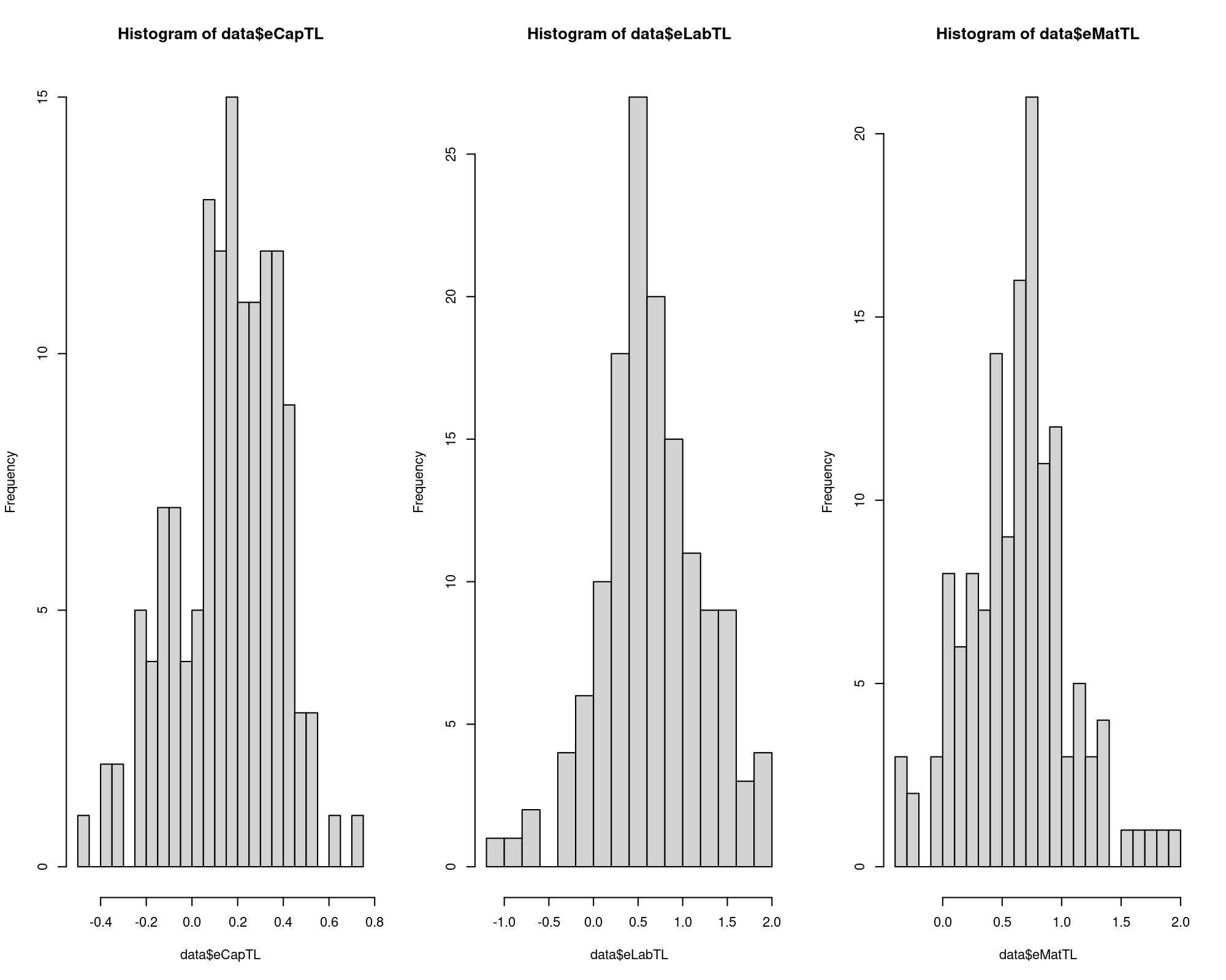
\(\Longrightarrow\) The median effect of an increase of 1% in an input has a positive median effect in the product (e.g. an increase of 1% in labour units increases the output in 0.6%), but the red flag here is that there are negative elasticities being them a sign of model misspecification.
And then I obtain the Marginal Productivity for the Translog Specification:
data$mpCapTL = with(data, eCapTL * qOutTL / qCap)
data$mpLabTL = with(data, eLabTL * qOutTL / qLab)
data$mpMatTL = with(data, eMatTL * qOutTL / qMat)

sum(data$mpCapTL < 0); sum(data$mpLabTL < 0); sum(data$mpMatTL < 0)

[1] 32

[1] 14

[1] 8

summary(data$mpCapTL); summary(data$mpLabTL); summary(data$mpMatTL)

   Min. 1st Qu.  Median    Mean 3rd Qu.    Max.
-13.681   0.534   3.766   4.566   7.369  26.836

   Min. 1st Qu.  Median    Mean 3rd Qu.    Max.
 -2.570   2.277   5.337   6.857  10.522  26.829

   Min. 1st Qu.  Median    Mean 3rd Qu.    Max.
 -28.44   28.55   51.83   48.12   70.97  122.86

par(mfrow=c(1,3)); hist(data$mpCapTL, breaks=20); hist(data$mpLabTL, breaks=20); hist(data$mpMatTL, breaks=20)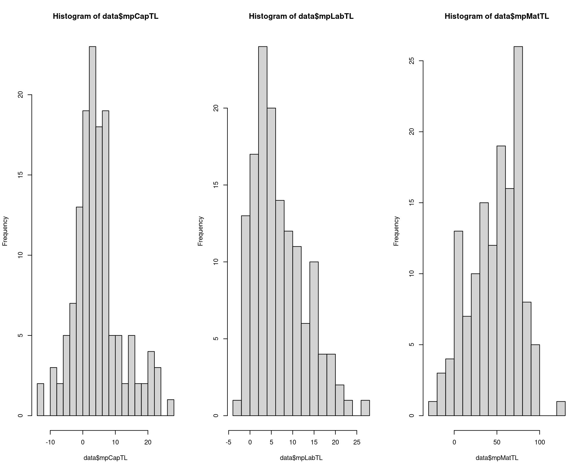
\(\Longrightarrow\) The effect of increasing the input in one unit has a positive median effect in the product (e.g. an increase of 1 labour unit increases the output in 5.3 units), but the red flag here is that there are negative marginal productivities being them another sign of model misspecification.
With the marginal productivity I can determine the number of observations that violate the monotonicity condition:
data$monoTL = with(data, mpCapTL >= 0 & mpLabTL >= 0 & mpMatTL >= 0 )
sum(!data$monoTL)

[1] 48
Now I compute the Scale Elasticity for the Translog Specification:
data$eScaleTL = data$eCapTL + data$eLabTL + data$eMatTL

sum(data$eScaleTL < 0)

[1] 0

summary(data$eScaleTL)

   Min. 1st Qu.  Median    Mean 3rd Qu.    Max.
  1.163   1.373   1.440   1.451   1.538   1.738

hist(data$eScaleTL, breaks=20)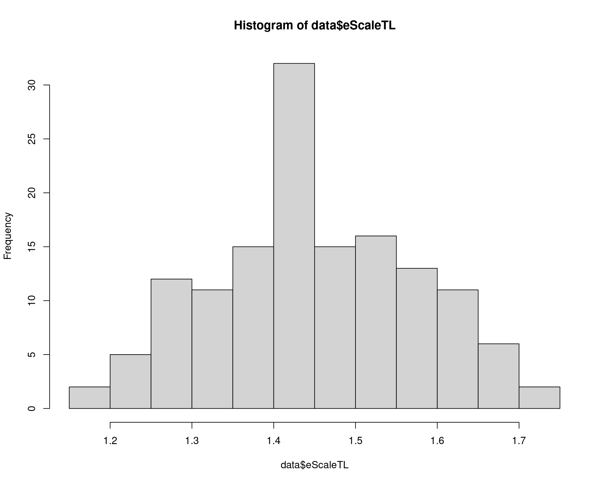
\(\Longrightarrow\) at least the Scale Elasticity is always positive, but there are negative Product-Factor Elasticities behind this result.
In the case of a Quadratic Specification the Marginal Productivity can be written as: \[MP_i = \beta_i + \sum_{j=1}^n \beta_{ij} x_j\] And from that I can obtain the Product-Factor Elasticity: \[\varepsilon_i = MP_i \frac{x_i}{y}\]
Now I compute the Marginal Productivity for the Quadratic Specification:
b1  = coef(prodQuad)["qCap"]
b2  = coef(prodQuad)["qLab"]
b3  = coef(prodQuad)["qMat"]
b11 = coef(prodQuad)["I(0.5 * qCap^2)"]
b22 = coef(prodQuad)["I(0.5 * qLab^2)"]
b33 = coef(prodQuad)["I(0.5 * qMat^2)"]
b12 = b21 = coef(prodQuad)["I(qCap * qLab)"]
b13 = b31 = coef(prodQuad)["I(qCap * qMat)"]
b23 = b32 = coef(prodQuad)["I(qLab * qMat)"]

data$mpCapQuad = with(data, b1 + b11*qCap + b12*qLab + b13*qMat)
data$mpLabQuad = with(data, b2 + b21*qCap + b22*qLab + b23*qMat)
data$mpMatQuad = with(data, b3 + b31*qCap + b32*qLab + b33*qMat)

sum(data$mpCapQuad < 0); sum(data$mpLabQuad < 0); sum(data$mpMatQuad < 0)

[1] 28

[1] 5

[1] 8

summary(data$mpCapQuad); summary(data$mpLabQuad); summary(data$mpMatQuad)

    Min.  1st Qu.   Median     Mean  3rd Qu.     Max.
-22.3351   0.7743   2.1523   1.7260   4.0267  16.6884

   Min. 1st Qu.  Median    Mean 3rd Qu.    Max.
 -1.599   4.224   6.113   7.031   9.513  30.780

   Min. 1st Qu.  Median    Mean 3rd Qu.    Max.
 -35.57   31.20   47.08   51.57   63.59  260.64

par(mfrow=c(1,3)); hist(data$mpCapQuad, breaks=20); hist(data$mpLabQuad, breaks=20); hist(data$mpMatQuad, breaks=20)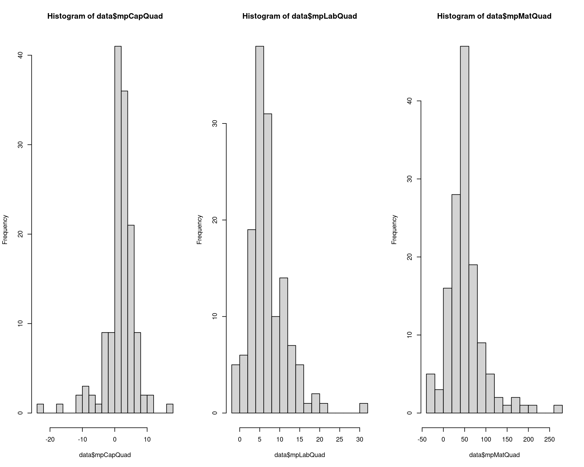
\(\Longrightarrow\) The effect of increasing the input in one unit has a positive median effect in the product (e.g. an increase of 1 labour unit increases the output in 6.1 units), but the red flag here is that there are negative marginal productivities being them another sign of model misspecification.
With the marginal productivity I can determine the number of observations that violate the monotonicity condition:
data$monoQuad = with(data, mpCapQuad >= 0 & mpLabQuad >= 0 & mpMatQuad >= 0 )
sum(!data$monoQuad)

[1] 39
And the Product-Factor Elasticity for the Quadratic Espcification:
data$eCapQuad = with(data, mpCapQuad * qCap / qOutQuad)
data$eLabQuad = with(data, mpLabQuad * qLab / qOutQuad)
data$eMatQuad = with(data, mpMatQuad * qMat / qOutQuad)

sum(data$eCapQuad < 0); sum(data$eLabQuad < 0); sum(data$eMatQuad < 0)

[1] 28

[1] 5

[1] 8


summary(data$eCapQuad); summary(data$eLabQuad); summary(data$eMatQuad)

    Min.  1st Qu.   Median     Mean  3rd Qu.     Max.
-0.34467  0.01521  0.07704  0.14240  0.21646  0.94331

   Min. 1st Qu.  Median    Mean 3rd Qu.    Max.
-0.3157  0.4492  0.6686  0.6835  0.8694  2.3563

   Min. 1st Qu.  Median    Mean 3rd Qu.    Max.
-1.4313  0.3797  0.5288  0.4843  0.6135  1.5114

par(mfrow=c(1,3)); hist(data$eCapQuad, breaks=20); hist(data$eLabQuad, breaks=20); hist(data$eMatQuad, breaks=20)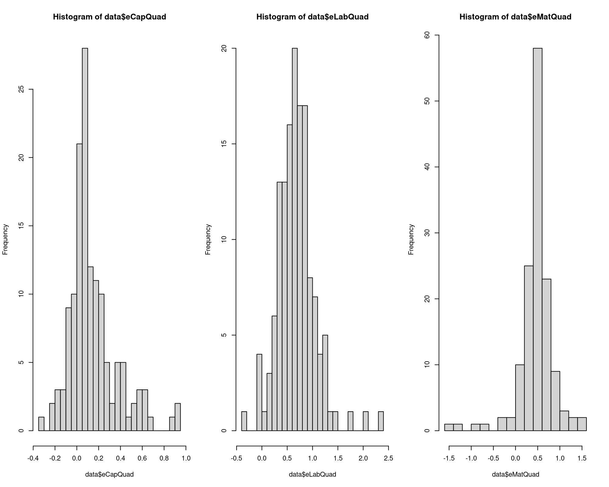
\(\Longrightarrow\) The median effect of an increase of 1% in an input has a positive median effect in the product (e.g. an increase of 1% in labour units increases the output in 0.67%), but the red flag here is that there are negative elasticities being them a sign of model misspecification.
Finally I compute the Scale Elasticity for the Quadratic Especification:
\(\Longrightarrow\) I should prefer the Translog Specification provided there are negative elasticities in this part.
Comparing both specifications:
| Quadratic | Translog | |
|---|---|---|
| \(R^2\) on \(y\) | 0.85 | 0.77 |
| \(R^2\) on \(ln(y)\) | 0.55 | 0.63 |
| Obs. with negative predicted output | 0 | 0 |
| Obs. that violate the monotonicity condition | 39 | 48 |
| Obs. with negative scale elasticity | 22 | 0 |
\(\Longrightarrow\) Translog Specification is not perfect but better than Quadratic Specification in this case. At leasts it has no negative scale elasticity. Both specifications violate the monotonicity condition for more than a 25% of the total observations, and this suggest both models are misspecified.
To seek for an accurate instrument to model the production I should go for a non-parametric regression. By doing that I do not depend on a functional form and I can work on a marginal effects basis that can solve the problem with negative effects of inputs increasing.