Contents of the talk

• Introduction

• API

• R Package

• Shiny Dashboard

• Code and documentation

Where to reach me

Twitter and Github: pachamaltese

Email: pacha # dcc * uchile * cl

Introduction

• Open Trade Statistics (OTS) was created with the intention to lower the barrier to working with international economic trade data.

• It includes a public API, a dashboard, and an R package for data retrieval.

Introduction

• Many Latin American Universities have limited or no access to the United Nations Commodity Trade Statistics Database (UN COMTRADE).

• This project shares curated datasets based on UN COMTRADE.

Introduction

The project has a major reproducibility flaw.

Introduction

Hardware and software stack

Introduction

The next three slides are an oversimplification just to explain the work in wide terms.

Introduction

The raw data contains missing flows:

Introduction

Possible solution (Anderson & van Wincoop, 2004 propose 8% rate):

Introduction

Customs have changed their coding systems in order to reflect changes in exported products (i.e. in 1960 nobody exported laptops).

Introduction

• We have 2018 data, similar initiatives have datasets updated to 2016 or 2017.

• But much more important than that, we converted all years to HS rev 2007 to allow time comparisons.

Comparison between APIs

Similar projects:

• The Atlas of Economic complexity (Harvard)
• The Obervatory of Economic complexity (it was from MIT)

Comparison between APIs

As a simple example, I shall compare three APIs by extracting what did Chile export to Argentina, Bolivia and Perú in 2016.

This shall be made by using common R packages:

library(jsonlite)
library(dplyr)
library(purrr)

Comparison between APIs

Open Trade Statistics

• docs.tradestatistics.io has fully detailed explanations to use the API

Comparison between APIs

Open Trade Statistics

# Function to read each combination reporter-partners
read_from_ots <- function(p) {
  fromJSON(sprintf("https://api.tradestatistics.io/yrpc?y=2016&r=chl&p=%s", p))
}
# The ISO codes are here: https://api.tradestatistics.io/countries
partners <- c("arg", "bol", "per")
# Now with purrr I can combine the three resulting datasets
# Chile-Argentina, Chile-Bolivia, and Chile-Perú
ots_data <- map_df(partners, read_from_ots)

Comparison between APIs

Open Trade Statistics

# Preview the data
as_tibble(ots_data)

## # A tibble: 2,767 x 6
##     year reporter_iso partner_iso product_code import_value_usd
##    <int> <chr>        <chr>       <chr>                   <int>
##  1  2016 chl          arg         2713                   430792
##  2  2016 chl          arg         2707                  5362832
##  3  2016 chl          arg         2705                     1405
##  4  2016 chl          arg         2704                  1506201
##  5  2016 chl          arg         2703                    20518
##  6  2016 chl          arg         2617                     4408
##  7  2016 chl          arg         2526                   147509
##  8  2016 chl          arg         2525                    10288
##  9  2016 chl          arg         2522                 54386957
## 10  2016 chl          arg         2521                    23209
## # … with 2,757 more rows, and 1 more variable: export_value_usd <int>

Comparison between APIs

Open Trade Statistics

# Product information
products <- fromJSON("https://api.tradestatistics.io/products")
# Join the two tables and then summarise by product group
# This will condense the original table into something more compact
# and even probably more informative
ots_data_2 <- ots_data %>%
  left_join(products, by = "product_code") %>%
  group_by(group_name) %>%
  summarise(export_value_usd = sum(export_value_usd, na.rm = T)) %>%
  arrange(-export_value_usd)

Comparison between APIs

Open Trade Statistics

ots_data_2

## # A tibble: 97 x 2
##    group_name                                              export_value_usd
##    <chr>                                                              <int>
##  1 Vehicles; other than railway or tramway rolling stock,…        443991154
##  2 Nuclear reactors, boilers, machinery and mechanical ap…        325689285
##  3 Electrical machinery and equipment and parts thereof; …        179255928
##  4 Plastics and articles thereof                                  171601876
##  5 Mineral fuels, mineral oils and products of their dist…        157105626
##  6 Iron or steel articles                                         152854400
##  7 Miscellaneous edible preparations                              149430227
##  8 Paper and paperboard; articles of paper pulp, of paper…        148626023
##  9 Fruit and nuts, edible; peel of citrus fruit or melons         138454388
## 10 Wood and articles of wood; wood charcoal                       113018698
## # … with 87 more rows

Comparison between APIs

The Observatory of Economic Complexity

• This API is documented at atlas.media.mit.edu/api.

• I'll try to replicate the result from OTS API.

Comparison between APIs

The Observatory of Economic Complexity

# Function to read each combination reporter-partners
read_from_oec <- function(p) {
  fromJSON(sprintf("https://atlas.media.mit.edu/hs07/export/2016/chl/%s/show/", p))
}
# From their documentation I can infer their links use ISO codes for countries,
# so I'll use the same codes from the previous example
destination <- c("arg", "bol", "per")
# One problem here is that the API returns a nested JSON that doesn't work with map_df
# I can obtain the same result with map and bind_rows
oec_data <- map(destination, read_from_oec)
oec_data <- bind_rows(oec_data[[1]]$data, oec_data[[2]]$data, oec_data[[3]]$data)

Comparison between APIs

The Observatory of Economic Complexity

oec_data %>% 
  select(dest_id, hs07_id, hs07_id_len, export_val) %>% 
  as_tibble()

## # A tibble: 9,933 x 4
##    dest_id hs07_id  hs07_id_len export_val
##    <chr>   <chr>          <dbl>      <dbl>
##  1 saarg   010101             6    455453.
##  2 saarg   01010110           8    100653.
##  3 saarg   01010190           8    354799.
##  4 saarg   010106             6        NA 
##  5 saarg   01010619           8        NA 
##  6 saarg   010201             6        NA 
##  7 saarg   01020130           8        NA 
##  8 saarg   010202             6        NA 
##  9 saarg   01020230           8        NA 
## 10 saarg   010204             6        NA 
## # … with 9,923 more rows

Comparison between APIs

The Observatory of Economic Complexity

Let's filter with this consideration in mind:

# Remember that this is a "false 6", and is a "4" actually
oec_data_2 <- oec_data %>%
  filter(hs07_id_len == 6) %>% 
  mutate(hs07_id = substr(hs07_id, 3, 6)) %>% 
  select(dest_id, hs07_id, export_val) %>% 
  as_tibble()

Comparison between APIs

The Observatory of Economic Complexity

oec_data_2

## # A tibble: 2,565 x 3
##    dest_id hs07_id export_val
##    <chr>   <chr>        <dbl>
##  1 saarg   0101       455453.
##  2 saarg   0106           NA 
##  3 saarg   0201           NA 
##  4 saarg   0202           NA 
##  5 saarg   0204           NA 
##  6 saarg   0206           NA 
##  7 saarg   0207           NA 
##  8 saarg   0302     36718891.
##  9 saarg   0303       211295.
## 10 saarg   0304     15793369.
## # … with 2,555 more rows

Comparison between APIs

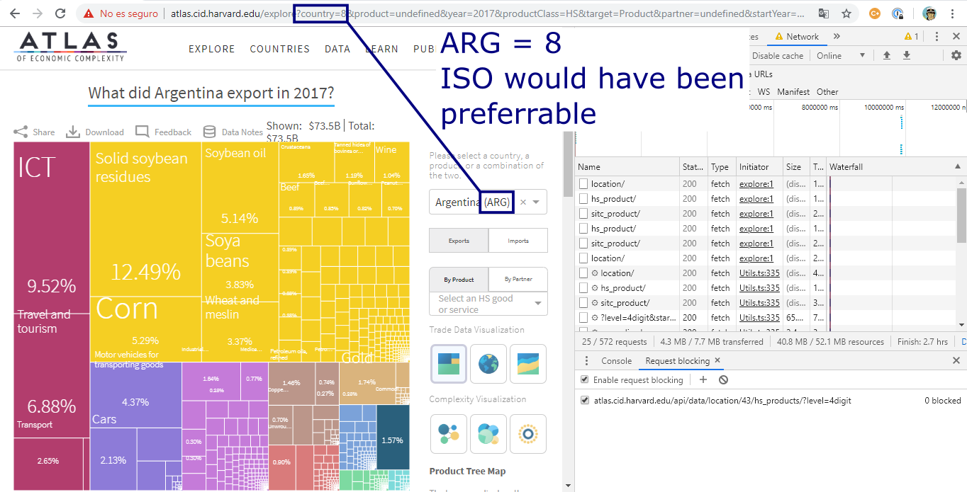
The Atlas of Economic Complexity

• I couldn't find documentation for this API

• Still I'll try to replicate the result from OTS API (I obtained the URL by using Firefox inspector at their website

Comparison between APIs

The Atlas of Economic Complexity

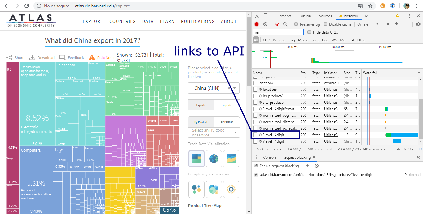
Comparison between APIs

The Atlas of Economic Complexity

Comparison between APIs

The Atlas of Economic Complexity

# Function to read each combination reporter-partners
read_from_atlas <- function(p) {
  fromJSON(sprintf("http://atlas.cid.harvard.edu/api/data/location/42/hs_products_by_partner/%s/?level=4digit", p))
}
# Getting to know these codes required web scraping from http://atlas.cid.harvard.edu/explore
# These codes don't follow UN COMTRADE numeric codes with are an alternative to ISO codes
destination <- c("8", "31", "173")
# The resulting JSON doesn't work with map_df either
# This can still be combined without much hassle
atlas_data <- map(destination, read_from_atlas)
atlas_data <- bind_rows(atlas_data[[1]]$data, atlas_data[[2]]$data, atlas_data[[3]]$data)

Comparison between APIs

The Atlas of Economic Complexity

atlas_data %>% 
  select(year, partner_id, product_id, export_value) %>% 
  as_tibble()

## # A tibble: 62,959 x 4
##     year partner_id product_id export_value
##    <int>      <int>      <int>        <int>
##  1  1995          8        650        23207
##  2  1996          8        650       152075
##  3  1997          8        650       131174
##  4  1998          8        650        64352
##  5  1999          8        650        78678
##  6  2000          8        650        85993
##  7  2001          8        650       500513
##  8  2002          8        650       191069
##  9  2003          8        650        89214
## 10  2004          8        650       242463
## # … with 62,949 more rows

Comparison between APIs

The Atlas of Economic Complexity

atlas_id_to_hs <- fromJSON("http://atlas.cid.harvard.edu/api/metadata/hs_product/")
atlas_id_to_hs <- atlas_id_to_hs$data %>% select(id, code)
atlas_id_to_iso <- fromJSON("http://atlas.cid.harvard.edu/api/metadata/location/")
atlas_id_to_iso <- atlas_id_to_iso$data %>% select(id, code)
atlas_data_2 <- atlas_data %>% 
  filter(year == 2016) %>%
  left_join(atlas_id_to_hs, by = c("product_id" = "id")) %>% 
  left_join(atlas_id_to_iso, by = c("partner_id" = "id"))

Comparison between APIs

The Atlas of Economic Complexity

atlas_data_2 %>%
  select(code.y, code.x, export_value) %>% 
  as_tibble()

## # A tibble: 2,705 x 3
##    code.y code.x export_value
##    <chr>  <chr>         <int>
##  1 ARG    0101         472353
##  2 ARG    0106              0
##  3 ARG    0201              0
##  4 ARG    0202              0
##  5 ARG    0204              0
##  6 ARG    0206              0
##  7 ARG    0207              0
##  8 ARG    0302       34514964
##  9 ARG    0303         214817
## 10 ARG    0304       14997462
## # … with 2,695 more rows

R package

# easy start
install.packages("tradestatistics")

R package

Fiji exports a lot of water. But how much of its exports to the US are actually water?

library(dplyr)
library(tradestatistics)
fji_usa <- ots_create_tidy_data(
  years = 2017, reporters = "fji", partners = "usa",
  include_shortnames = T
)
fji_usa_2 <- fji_usa %>% 
  select(product_shortname_english, export_value_usd) %>% 
  arrange(-export_value_usd) %>% 
  mutate(export_value_share = round(100 * export_value_usd /
                                      sum(export_value_usd, na.rm = T), 2))

R package

fji_usa_2

## # A tibble: 736 x 3
##    product_shortname_english export_value_usd export_value_share
##    <chr>                                <int>              <dbl>
##  1 Water                            233431002              60   
##  2 Processed Fish                    61666883              15.8 
##  3 Non-fillet Fresh Fish             18503975               4.76
##  4 Raw Sugar                         12600118               3.24
##  5 Broadcasting Equipment            10967992               2.82
##  6 Perfume Plants                     7273321               1.87
##  7 Fish Fillets                       5540948               1.42
##  8 Unspecified                        4246687               1.09
##  9 Non-fillet Frozen Fish             4033516               1.04
## 10 Molasses                           3578212               0.92
## # … with 726 more rows

R package

Which country from America is the #1 partner with the European Union (EU-28)?

eu28 <- ots_countries %>% 
  filter(eu28_member == 1) %>% 
  select(country_iso)
ame_eu28 <- ots_create_tidy_data(
  years = 2017, reporters = "c-am", partners = "all",
  table = "yrp"
)

ame_eu28_2 <- ame_eu28 %>% 
  mutate(is_eu28 = ifelse(partner_iso %in% eu28$country_iso, 1, 0)) %>% 
  group_by(reporter_iso, is_eu28) %>% 
  summarise(export_value_usd = sum(export_value_usd, na.rm = T)) %>% 
  group_by(reporter_iso) %>%
  mutate(pct_to_eu28 = export_value_usd / sum(export_value_usd, na.rm = T)) %>% 
  filter(is_eu28 == 1) %>% 
  select(reporter_iso, export_value_usd, pct_to_eu28) %>% 
  arrange(-export_value_usd)

ame_eu28_2

## # A tibble: 48 x 3
## # Groups:   reporter_iso [48]
##    reporter_iso export_value_usd pct_to_eu28
##    <chr>                   <dbl>       <dbl>
##  1 usa              406704170165      0.218 
##  2 can               51259679792      0.109 
##  3 bra               45042481104      0.174 
##  4 mex               34405957170      0.0711
##  5 chl               10937519973      0.144 
##  6 arg               10872575385      0.165 
##  7 per                8375757038      0.170 
##  8 col                8124020268      0.168 
##  9 cri                3922634462      0.246 
## 10 ecu                3917486407      0.169 
## # … with 38 more rows

Dashboard

shiny.tradestatistics.io

Code and documentation

github.com/tradestatistics

docs.ropensci.org/tradestatistics

tradestatistics.io

Related packages

• Gravity (CRAN): Complex econometric models for international trade
• Economiccomplexity (CRAN): Recursive methods for international trade

Acknowledgements

• rOpenSci <3: Amanda, Emily, Jorge, Maelle, Mark and Stefanie
• DigitalOcean: Danny
• Highcharter/Design: Joshua and Erasmo