CP 1919 / PSR B1919+21 Dataset

aka Joy Division’s plot

If you like these contributions, please consider buying me a coffee.

About

I added the CP 1919 / PSR B1919+21 Dataset to my GitHub.

This dataset, found in one of my old external drives, corresponds to the famous plot from Radio Observations of the Pulse Profiles and Dispersion Measures of Twelve Pulsars (Craft, 1970). This is broadly known as the Joy Division’s plot from Unknown Pleasures. If you happen to know whom created the provided CSV file, please let me know so I can give proper credit.

The dataset contains “successive pulses from the first pulsar discovered, CP 1919, are here superimposed vertically. The pulses occur every 1.337 seconds. They are caused by rapidly spinning neutron star.” (The Cambridge Encyclopaedia of Astronomy, 1977)

Thanks to Scientific American, there is a complete explanation of the dataset and its origin.

Read

pulsar <- readr::read_csv("https://raw.githubusercontent.com/pachadotdev/cp1919/main/cp1919.csv")

Rows: 24000 Columns: 3
── Column specification ────────────────────────────────────────────────────────
Delimiter: ","
dbl (3): x, y, z

ℹ Use `spec()` to retrieve the full column specification for this data.
ℹ Specify the column types or set `show_col_types = FALSE` to quiet this message.

pulsar

# A tibble: 24,000 × 3
       x     y     z
   <dbl> <dbl> <dbl>
 1     1     1 -0.81
 2     2     1 -0.91
 3     3     1 -1.09
 4     4     1 -1   
 5     5     1 -0.59
 6     6     1 -0.82
 7     7     1 -0.43
 8     8     1 -0.68
 9     9     1 -0.71
10    10     1 -0.27
# ℹ 23,990 more rows

Visualize

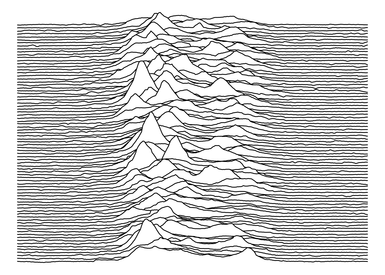
The Cambridge Encyclopaedia of Astronomy (1977)

library(ggplot2)
library(ggridges)

col1 <- "white"
col2 <- "black"

ggplot(pulsar, aes(x = x, y = y, height = z, group = y)) +
  geom_ridgeline(
    min_height = min(pulsar$z),
    scale = 0.2,
    linewidth = 0.5,
    fill = col1,
    colour = col2
  ) +
  scale_y_reverse() +
  theme_void() +
  theme(
    panel.background = element_rect(fill = col1),
    plot.background = element_rect(fill = col1, color = col1),
  )

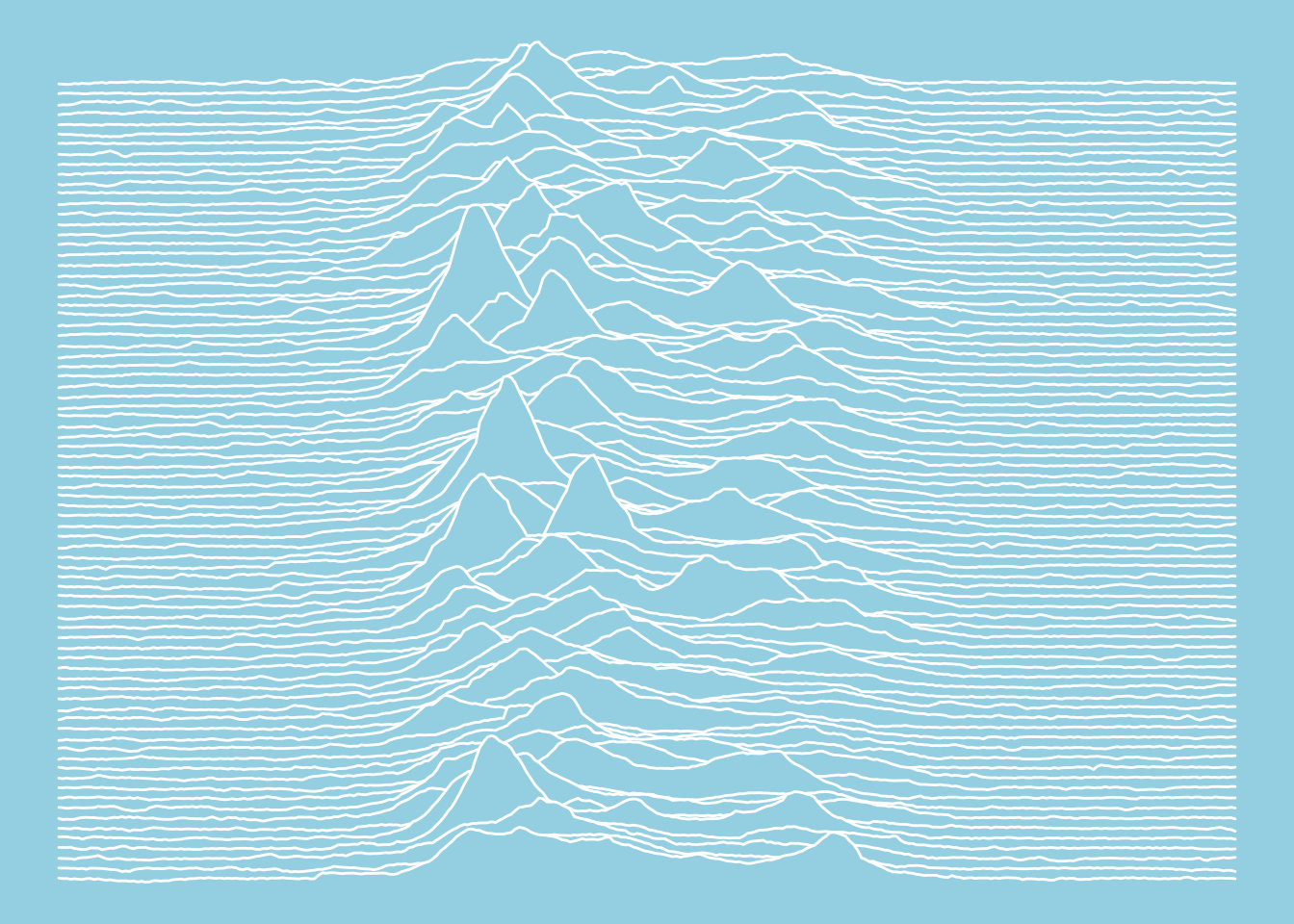
The Nature of Pulsars (Scientific American, 1970)

col1 <- "#94cee1"
col2 <- "white"

ggplot(pulsar, aes(x = x, y = y, height = z, group = y)) +
  geom_ridgeline(
    min_height = min(pulsar$z),
    scale = 0.2,
    linewidth = 0.5,
    fill = col1,
    colour = col2
  ) +
  scale_y_reverse() +
  theme_void() +
  theme(
    panel.background = element_rect(fill = col1),
    plot.background = element_rect(fill = col1, color = col1),
  )

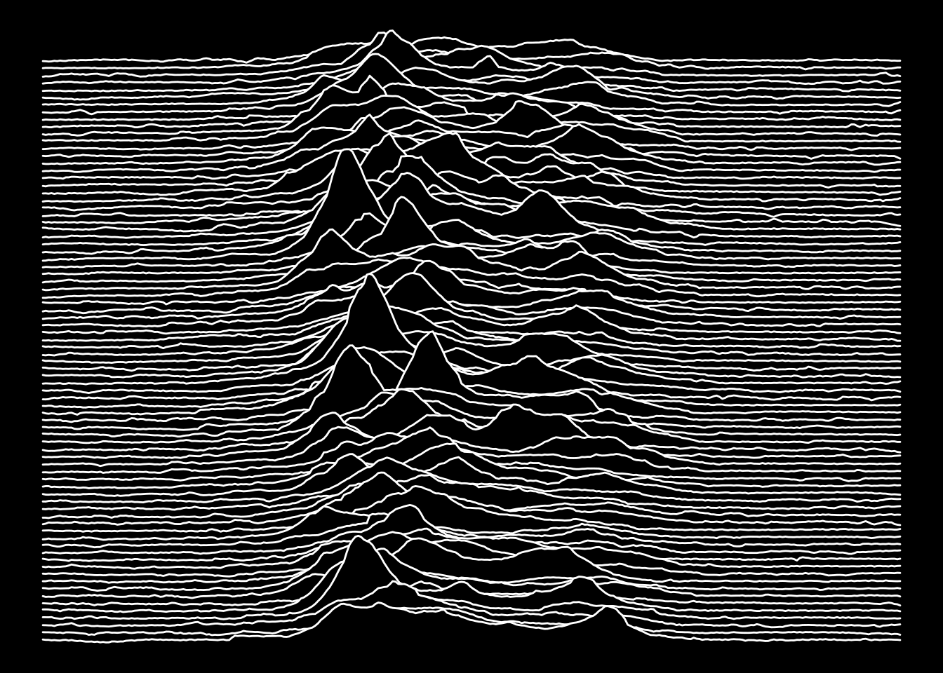
Joy Division’s Unknown Pleasures (1979)

col1 <- "black"
col2 <- "white"

ggplot(pulsar, aes(x = x, y = y, height = z, group = y)) +
  geom_ridgeline(
    min_height = min(pulsar$z),
    scale = 0.2,
    linewidth = 0.5,
    fill = col1,
    colour = col2
  ) +
  scale_y_reverse() +
  theme_void() +
  theme(
    panel.background = element_rect(fill = col1),
    plot.background = element_rect(fill = col1, color = col1),
  )